2014-05-04 22:57:02 +00:00
{
"metadata": {
"name": "",
2014-05-10 16:05:43 +00:00
"signature": "sha256:5d04280c23460c2481423dabf313f3ad28f40fb4ad915967d83e3a08231c8b3d"
2014-05-04 22:57:02 +00:00
},
"nbformat": 3,
"nbformat_minor": 0,
"worksheets": [
{
"cells": [
{
"cell_type": "markdown",
"metadata": {},
"source": [
2014-05-05 00:16:02 +00:00
"[Sebastian Raschka](http://www.sebastianraschka.com) \n",
2014-05-10 00:28:22 +00:00
"last updated: 05/09/2014\n",
2014-05-04 22:57:02 +00:00
"\n",
2014-05-04 23:11:16 +00:00
"- [Link to this IPython Notebook on GitHub](https://github.com/rasbt/python_reference/blob/master/benchmarks/cython_least_squares.ipynb) \n",
2014-05-04 22:57:02 +00:00
"- [Link to the GitHub repository](https://github.com/rasbt/python_reference)"
]
},
{
"cell_type": "markdown",
"metadata": {},
"source": [
2014-05-05 19:34:22 +00:00
"#### The code in this notebook was executed in Python 3.4.0"
2014-05-04 22:57:02 +00:00
]
},
{
"cell_type": "markdown",
"metadata": {},
"source": [
"<hr>\n",
"I am really looking forward to your comments and suggestions to improve and \n",
"extend this little collection! Just send me a quick note \n",
"via Twitter: [@rasbt](https://twitter.com/rasbt) \n",
"or Email: [bluewoodtree@gmail.com](mailto:bluewoodtree@gmail.com)\n",
"<hr>"
]
},
{
"cell_type": "markdown",
"metadata": {},
"source": [
"# Implementing the least squares fit method for linear regression and speeding it up via Cython"
]
},
{
"cell_type": "markdown",
"metadata": {},
"source": [
"<a name=\"sections\"></a>\n",
"<br>\n",
"<br>\n"
]
},
{
"cell_type": "markdown",
"metadata": {},
"source": [
"#Sections"
]
},
{
"cell_type": "markdown",
"metadata": {},
"source": [
"- [Introduction](#introduction)\n",
"- [Least squares fit implementations](#implementations)\n",
2014-05-10 00:28:22 +00:00
" - [1. The matrix approach in (C)Python and NumPy](#matrix_approach)\n",
" - [2. The classic approach in (C)Python, Cython, and Numba](#classic_approach)\n",
" - [3. Using the `numpy.linalg.lstsq` function](#numpy_func)\n",
" - [4. Using the `scipy.stats.linregress` function](#scipy_func)\n",
2014-05-04 22:57:02 +00:00
"- [Generating sample data and benchmarking](#sample_data)\n",
2014-05-10 00:28:22 +00:00
" - [Performance growth rates: (C)Python vs. Cython vs. Numba](#performance1)\n",
" - [Performance growth rates: NumPy and SciPy library functions](#performance2)\n",
"- [Bonus: How to use Cython without the IPython magic](#cython_bonus)"
2014-05-04 22:57:02 +00:00
]
},
{
"cell_type": "markdown",
"metadata": {},
"source": [
"<a name=\"introduction\"></a>\n",
"<br>\n",
"<br>"
]
},
2014-05-05 19:34:22 +00:00
{
"cell_type": "markdown",
"metadata": {},
"source": [
2014-05-06 18:38:02 +00:00
"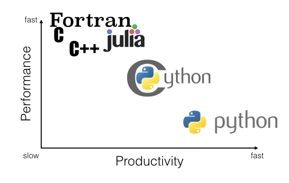 \n",
2014-05-05 19:34:22 +00:00
"(Note that this chart just reflects my rather objective thoughts after experimenting with Cython, and it is not based on real numbers or benchmarks.)\n",
"<br>\n",
"<br>\n",
"<br>\n",
"<br>"
]
},
2014-05-04 22:57:02 +00:00
{
"cell_type": "markdown",
"metadata": {},
"source": [
2014-05-10 00:28:22 +00:00
"# Introduction"
2014-05-04 22:57:02 +00:00
]
},
{
"cell_type": "markdown",
"metadata": {},
"source": [
"[[back to top](#sections)]"
]
},
{
"cell_type": "markdown",
"metadata": {},
"source": [
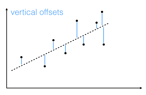
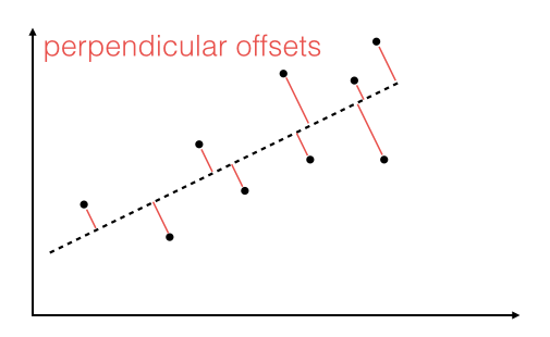
"Linear regression via the least squares method is the simplest approach to performing a regression analysis of a dependent and a explanatory variable. The objective is to find the best-fitting straight line through a set of points that minimizes the sum of the squared offsets from the line. \n",
"The offsets come in 2 different flavors: perpendicular and vertical - with respect to the line. \n",
" \n",
" \n",
"\n",
2014-05-05 02:17:27 +00:00
"As Michael Burger summarizes it nicely in his article \"[Problems of Linear Least Square Regression - And Approaches to Handle Them](http://www.arsa-conf.com/archive/?vid=1&aid=2&kid=60101-220)\": \"the perpendicular offset method delivers a more precise result but is are more complicated to handle. Therefore normally the vertical offsets are used.\" \n",
"Here, we will also use the method of computing the vertical offsets.\n",
"\n"
2014-05-04 22:57:02 +00:00
]
},
{
"cell_type": "markdown",
"metadata": {},
"source": [
"In more mathematical terms, our goal is to compute the best fit to *n* points $(x_i, y_i)$ with $i=1,2,...n,$ via linear equation of the form \n",
"$f(x) = a\\cdot x + b$. \n",
2014-05-06 18:38:02 +00:00
"We further have to assume that the y-component is functionally dependent on the x-component. \n",
2014-05-04 22:57:02 +00:00
"In a cartesian coordinate system, $b$ is the intercept of the straight line with the y-axis, and $a$ is the slope of this line."
]
},
{
"cell_type": "markdown",
"metadata": {},
"source": [
"In order to obtain the parameters for the linear regression line for a set of multiple points, we can re-write the problem as matrix equation \n",
"$\\pmb X \\; \\pmb a = \\pmb y$"
]
},
{
"cell_type": "markdown",
"metadata": {},
"source": [
"$\\Rightarrow\\Bigg[ \\begin{array}{cc}\n",
"x_1 & 1 \\\\\n",
"... & 1 \\\\\n",
"x_n & 1 \\end{array} \\Bigg]$\n",
"$\\bigg[ \\begin{array}{c}\n",
"a \\\\\n",
"b \\end{array} \\bigg]$\n",
"$=\\Bigg[ \\begin{array}{c}\n",
"y_1 \\\\\n",
"... \\\\\n",
"y_n \\end{array} \\Bigg]$"
]
},
{
"cell_type": "markdown",
"metadata": {},
"source": [
"With a little bit of calculus, we can rearrange the term in order to obtain the parameter vector $\\pmb a = [a\\;b]^T$"
]
},
{
"cell_type": "markdown",
"metadata": {},
"source": [
"$\\Rightarrow \\pmb a = (\\pmb X^T \\; \\pmb X)^{-1} \\pmb X^T \\; \\pmb y$"
]
},
{
"cell_type": "markdown",
"metadata": {},
"source": [
"<br>\n",
"The more classic approach to obtain the slope parameter $a$ and y-axis intercept $b$ would be:"
]
},
{
"cell_type": "markdown",
"metadata": {},
"source": [
"$a = \\frac{S_{x,y}}{\\sigma_{x}^{2}}\\quad$ (slope)\n",
"\n",
"\n",
"$b = \\bar{y} - a\\bar{x}\\quad$ (y-axis intercept)"
]
},
{
"cell_type": "markdown",
"metadata": {},
"source": [
"where \n",
"\n",
"\n",
"$S_{xy} = \\sum_{i=1}^{n} (x_i - \\bar{x})(y_i - \\bar{y})\\quad$ (covariance)\n",
"\n",
"\n",
"$\\sigma{_x}^{2} = \\sum_{i=1}^{n} (x_i - \\bar{x})^2\\quad$ (variance)"
]
},
{
"cell_type": "markdown",
"metadata": {},
"source": [
"<a name=\"implementations\"></a>\n",
"<br>\n",
"<br>"
]
},
{
"cell_type": "markdown",
"metadata": {},
"source": [
"\n",
2014-05-10 00:28:22 +00:00
"# Least squares fit implementations"
2014-05-04 22:57:02 +00:00
]
},
{
"cell_type": "markdown",
"metadata": {},
"source": [
"[[back to top](#sections)]"
]
},
{
"cell_type": "markdown",
"metadata": {},
"source": [
2014-05-10 00:28:22 +00:00
"<a name='matrix_approach'></a>\n",
2014-05-04 22:57:02 +00:00
"<br>\n",
"<br>"
]
},
{
"cell_type": "markdown",
"metadata": {},
"source": [
2014-05-10 00:28:22 +00:00
"### 1. The matrix approach in (C)Python and NumPy"
]
},
{
"cell_type": "markdown",
"metadata": {},
"source": [
"[[back to top](#sections)]"
2014-05-04 22:57:02 +00:00
]
},
{
"cell_type": "markdown",
"metadata": {},
"source": [
"First, let us implement the equation:"
]
},
{
"cell_type": "markdown",
"metadata": {},
"source": [
"$\\pmb a = (\\pmb X^T \\; \\pmb X)^{-1} \\pmb X^T \\; \\pmb y$"
]
},
{
"cell_type": "markdown",
"metadata": {},
"source": [
"which I will refer to as the \"matrix approach\"."
]
},
2014-05-10 00:28:22 +00:00
{
"cell_type": "markdown",
"metadata": {},
"source": [
"#### Matrix approach implemented in NumPy and (C)Python"
]
},
2014-05-04 22:57:02 +00:00
{
"cell_type": "code",
"collapsed": false,
"input": [
"import numpy as np\n",
"\n",
2014-05-10 00:28:22 +00:00
"def py_matrix_lstsqr(x, y):\n",
2014-05-04 22:57:02 +00:00
" \"\"\" Computes the least-squares solution to a linear matrix equation. \"\"\"\n",
" X = np.vstack([x, np.ones(len(x))]).T\n",
" return (np.linalg.inv(X.T.dot(X)).dot(X.T)).dot(y)"
],
"language": "python",
"metadata": {},
"outputs": [],
2014-05-10 16:05:43 +00:00
"prompt_number": 9
2014-05-04 22:57:02 +00:00
},
{
"cell_type": "markdown",
"metadata": {},
"source": [
2014-05-10 00:28:22 +00:00
"<a name='classic_approach'></a>\n",
2014-05-04 22:57:02 +00:00
"<br>\n",
"<br>"
]
},
{
"cell_type": "markdown",
"metadata": {},
"source": [
2014-05-10 00:28:22 +00:00
"### 2. The classic approach in (C)Python, Cython, and Numba"
]
},
{
"cell_type": "markdown",
"metadata": {},
"source": [
"[[back to top](#sections)]"
2014-05-04 22:57:02 +00:00
]
},
{
"cell_type": "markdown",
"metadata": {},
"source": [
2014-05-06 18:38:02 +00:00
"Next, we will calculate the parameters separately, using standard library functions in Python only, which I will call the \"classic approach\"."
2014-05-04 22:57:02 +00:00
]
},
{
"cell_type": "markdown",
"metadata": {},
"source": [
"$a = \\frac{S_{x,y}}{\\sigma_{x}^{2}}\\quad$ (slope)\n",
"\n",
"\n",
"$b = \\bar{y} - a\\bar{x}\\quad$ (y-axis intercept)"
]
},
2014-05-10 00:28:22 +00:00
{
"cell_type": "markdown",
"metadata": {},
"source": [
"Note: I refrained from using list comprehensions and convenience functions such as `zip()` in\n",
"order to maximize the performance for the Cython compilation into C code in the later sections.\n",
" "
]
},
{
"cell_type": "markdown",
"metadata": {},
"source": [
"#### Implemented in (C)Python"
]
},
2014-05-04 22:57:02 +00:00
{
"cell_type": "code",
"collapsed": false,
"input": [
2014-05-10 00:28:22 +00:00
"def py_classic_lstsqr(x, y):\n",
2014-05-04 22:57:02 +00:00
" \"\"\" Computes the least-squares solution to a linear matrix equation. \"\"\"\n",
2014-05-10 00:28:22 +00:00
" len_x = len(x)\n",
" x_avg = sum(x)/len_x\n",
2014-05-04 22:57:02 +00:00
" y_avg = sum(y)/len(y)\n",
2014-05-10 00:28:22 +00:00
" var_x = 0\n",
" cov_xy = 0\n",
" for i in range(len_x):\n",
" temp = (x[i] - x_avg)\n",
" var_x += temp**2\n",
" cov_xy += temp*(y[i] - y_avg)\n",
2014-05-04 22:57:02 +00:00
" slope = cov_xy / var_x\n",
" y_interc = y_avg - slope*x_avg\n",
2014-05-10 00:28:22 +00:00
" return (slope, y_interc) "
2014-05-04 22:57:02 +00:00
],
"language": "python",
"metadata": {},
"outputs": [],
2014-05-10 16:05:43 +00:00
"prompt_number": 1
2014-05-04 22:57:02 +00:00
},
{
"cell_type": "markdown",
"metadata": {},
"source": [
2014-05-10 00:28:22 +00:00
"#### Implemented in Cython"
2014-05-04 22:57:02 +00:00
]
},
{
"cell_type": "markdown",
"metadata": {},
"source": [
2014-05-10 00:28:22 +00:00
"Maybe we can speed things up a little bit via [Cython's C-extensions for Python](http://cython.org). Cython is basically a hybrid between C and Python and can be pictured as compiled Python code with type declarations. \n",
"Since we are working in an IPython notebook here, we can make use of the very convenient *IPython magic*: It will take care of the conversion to C code, the compilation, and eventually the loading of the function. "
2014-05-04 22:57:02 +00:00
]
},
{
"cell_type": "code",
"collapsed": false,
"input": [
2014-05-10 00:28:22 +00:00
"%load_ext cythonmagic"
2014-05-04 22:57:02 +00:00
],
"language": "python",
"metadata": {},
"outputs": [],
2014-05-10 16:05:43 +00:00
"prompt_number": 2
2014-05-04 22:57:02 +00:00
},
{
2014-05-10 00:28:22 +00:00
"cell_type": "code",
"collapsed": false,
"input": [
"%%cython\n",
"def cy_classic_lstsqr(x, y):\n",
" \"\"\" Computes the least-squares solution to a linear matrix equation. \"\"\"\n",
" cdef double x_avg, y_avg, var_x, cov_xy,\\\n",
" slope, y_interc, x_i, y_i\n",
" cdef int len_x\n",
" len_x = len(x)\n",
" x_avg = sum(x)/len_x\n",
" y_avg = sum(y)/len(y)\n",
" var_x = 0\n",
" cov_xy = 0\n",
" for i in range(len_x):\n",
" temp = (x[i] - x_avg)\n",
" var_x += temp**2\n",
" cov_xy += temp*(y[i] - y_avg)\n",
" slope = cov_xy / var_x\n",
" y_interc = y_avg - slope*x_avg\n",
" return (slope, y_interc)"
],
"language": "python",
2014-05-04 22:57:02 +00:00
"metadata": {},
2014-05-10 00:28:22 +00:00
"outputs": [],
2014-05-10 16:05:43 +00:00
"prompt_number": 3
2014-05-04 22:57:02 +00:00
},
{
"cell_type": "markdown",
"metadata": {},
"source": [
2014-05-10 00:28:22 +00:00
"#### Implemented in Numba"
2014-05-04 22:57:02 +00:00
]
},
{
"cell_type": "markdown",
"metadata": {},
"source": [
2014-05-10 00:28:22 +00:00
"Like we did with Cython before, we will use the minimalist approach to Numba and see how the two - Cython and Numba - compare against each other. \n",
"\n",
"Numba is using the [LLVM compiler infrastructure](http://llvm.org) for compiling Python code to machine code. Its strength is to work with NumPy arrays to speed-up the code. If you want to read more about Numba, please see refer to the original [website and documentation](http://numba.pydata.org/numba-doc/0.13/index.html)."
2014-05-04 22:57:02 +00:00
]
},
{
"cell_type": "code",
"collapsed": false,
"input": [
2014-05-10 00:28:22 +00:00
"from numba import jit\n",
2014-05-04 22:57:02 +00:00
"\n",
2014-05-10 00:28:22 +00:00
"@jit\n",
"def numba_classic_lstsqr(x, y):\n",
2014-05-04 22:57:02 +00:00
" \"\"\" Computes the least-squares solution to a linear matrix equation. \"\"\"\n",
2014-05-10 00:28:22 +00:00
" len_x = len(x)\n",
" x_avg = sum(x)/len_x\n",
" y_avg = sum(y)/len(y)\n",
" var_x = 0\n",
" cov_xy = 0\n",
" for i in range(len_x):\n",
" temp = (x[i] - x_avg)\n",
" var_x += temp**2\n",
" cov_xy += temp*(y[i] - y_avg)\n",
" slope = cov_xy / var_x\n",
" y_interc = y_avg - slope*x_avg\n",
" return (slope, y_interc)"
2014-05-04 22:57:02 +00:00
],
"language": "python",
"metadata": {},
"outputs": [],
2014-05-10 16:05:43 +00:00
"prompt_number": 4
2014-05-06 18:38:02 +00:00
},
{
"cell_type": "markdown",
"metadata": {},
"source": [
2014-05-10 00:28:22 +00:00
"<a name='numpy_func'></a>\n",
2014-05-06 18:38:02 +00:00
"<br>\n",
"<br>"
]
},
{
"cell_type": "markdown",
"metadata": {},
"source": [
2014-05-10 00:28:22 +00:00
"### 3. Using the `numpy.linalg.lstsq` function"
2014-05-06 18:38:02 +00:00
]
},
{
"cell_type": "markdown",
"metadata": {},
"source": [
2014-05-10 00:28:22 +00:00
"[[back to top](#sections)]"
2014-05-06 18:38:02 +00:00
]
2014-05-04 22:57:02 +00:00
},
{
"cell_type": "markdown",
"metadata": {},
"source": [
2014-05-10 00:28:22 +00:00
"For our convenience, `numpy` has a function that can computes the least squares solution of a linear matrix equation. For more information, please refer to the [documentation](http://docs.scipy.org/doc/numpy/reference/generated/numpy.linalg.lstsq.html)."
]
},
{
"cell_type": "code",
"collapsed": false,
"input": [
"def numpy_lstsqr(x, y):\n",
" \"\"\" Computes the least-squares solution to a linear matrix equation. \"\"\"\n",
" X = np.vstack([x, np.ones(len(x))]).T\n",
" return np.linalg.lstsq(X,y)[0]"
],
"language": "python",
"metadata": {},
"outputs": [],
2014-05-10 16:05:43 +00:00
"prompt_number": 5
2014-05-10 00:28:22 +00:00
},
{
"cell_type": "markdown",
"metadata": {},
"source": [
"<a name='scipy_func'></a>\n",
2014-05-04 22:57:02 +00:00
"<br>\n",
"<br>"
]
},
{
"cell_type": "markdown",
"metadata": {},
"source": [
2014-05-10 00:28:22 +00:00
"### 4. Using the `scipy.stats.linregress` function"
2014-05-04 22:57:02 +00:00
]
},
{
"cell_type": "markdown",
"metadata": {},
"source": [
"[[back to top](#sections)]"
]
},
{
"cell_type": "markdown",
"metadata": {},
"source": [
2014-05-10 00:28:22 +00:00
"Also scipy has a least squares function, `scipy.stats.linregress()`, which returns a tuple of 5 different attributes, where the 1st value in the tuple is the slope, and the second value is the y-axis intercept, respectively. \n",
"The documentation for this function can be found [here](http://docs.scipy.org/doc/scipy-0.13.0/reference/generated/scipy.stats.linregress.html)."
2014-05-04 22:57:02 +00:00
]
},
{
"cell_type": "code",
"collapsed": false,
"input": [
2014-05-10 00:28:22 +00:00
"import scipy.stats\n",
2014-05-04 22:57:02 +00:00
"\n",
2014-05-10 00:28:22 +00:00
"def scipy_lstsqr(x,y):\n",
" \"\"\" Computes the least-squares solution to a linear matrix equation. \"\"\"\n",
" return scipy.stats.linregress(x, y)[0:2]"
2014-05-04 22:57:02 +00:00
],
"language": "python",
"metadata": {},
"outputs": [],
2014-05-10 16:05:43 +00:00
"prompt_number": 6
2014-05-10 00:28:22 +00:00
},
{
"cell_type": "markdown",
"metadata": {},
"source": [
"<br>\n",
"<br>"
]
},
{
"cell_type": "markdown",
"metadata": {},
"source": [
"<a name='sample_data'></a>\n",
"<br>\n",
"<br>"
]
},
{
"cell_type": "markdown",
"metadata": {},
"source": [
"# Generating sample data and benchmarking"
]
},
{
"cell_type": "markdown",
"metadata": {},
"source": [
"[[back to top](#sections)]"
]
2014-05-04 22:57:02 +00:00
},
{
"cell_type": "markdown",
"metadata": {},
"source": [
"<br>\n",
2014-05-04 23:21:25 +00:00
"<br>"
]
},
{
"cell_type": "markdown",
"metadata": {},
"source": [
"\n",
2014-05-04 22:57:02 +00:00
"#### Visualization"
]
},
{
"cell_type": "markdown",
"metadata": {},
"source": [
2014-05-06 18:38:02 +00:00
"To check how our dataset is distributed, and how the least squares regression line looks like, we will plot the results in a scatter plot. \n",
"Note that we are only using our \"matrix approach\" to visualize the results - for simplicity. We expect all 4 approaches to produce similar results, which we will confirm after visualizing the data."
2014-05-04 22:57:02 +00:00
]
},
{
"cell_type": "code",
"collapsed": false,
"input": [
2014-05-10 00:28:22 +00:00
"%matplotlib inline"
2014-05-06 18:38:02 +00:00
],
"language": "python",
"metadata": {},
"outputs": [],
2014-05-10 16:05:43 +00:00
"prompt_number": 7
2014-05-06 18:38:02 +00:00
},
{
"cell_type": "code",
"collapsed": false,
"input": [
2014-05-04 22:57:02 +00:00
"from matplotlib import pyplot as plt\n",
2014-05-10 00:28:22 +00:00
"import random\n",
"\n",
"random.seed(12345)\n",
2014-05-04 22:57:02 +00:00
"\n",
2014-05-10 00:28:22 +00:00
"x = [x_i*random.randrange(8,12)/10 for x_i in range(500)]\n",
"y = [y_i*random.randrange(8,12)/10 for y_i in range(100,600)]\n",
"\n",
"slope, intercept = py_matrix_lstsqr(x, y)\n",
2014-05-04 22:57:02 +00:00
"\n",
"line_x = [round(min(x)) - 1, round(max(x)) + 1]\n",
"line_y = [slope*x_i + intercept for x_i in line_x]\n",
"\n",
"plt.figure(figsize=(8,8))\n",
"plt.scatter(x,y)\n",
"plt.plot(line_x, line_y, color='red', lw='2')\n",
"\n",
"plt.ylabel('y')\n",
"plt.xlabel('x')\n",
"plt.title('Linear regression via least squares fit')\n",
"\n",
"ftext = 'y = ax + b = {:.3f} + {:.3f}x'\\\n",
" .format(slope, intercept)\n",
"plt.figtext(.15,.8, ftext, fontsize=11, ha='left')\n",
"\n",
"plt.show()"
],
"language": "python",
"metadata": {},
"outputs": [
{
"metadata": {},
"output_type": "display_data",
"png": "iVBORw0KGgoAAAANSUhEUgAAAfoAAAH4CAYAAACi3S9CAAAABHNCSVQICAgIfAhkiAAAAAlwSFlz\nAAALEgAACxIB0t1+/AAAIABJREFUeJzs3XdUVMfbwPHv0lm6giAgooBRbNi7GCv2EnvXWOPPnhg1\nGksSxRhjoiYaE0SNsb4xEY0Fe+zGmijGLkZARRERFljYnfeP1Y0ELJRlAedzDkf2lpln7q48e++d\nO6MQQggkSZIkSSqSTIwdgCRJkiRJhiMTvSRJkiQVYTLRS5IkSVIRJhO9JEmSJBVhMtFLkiRJUhEm\nE70kSZIkFWEy0UtGd+jQIcqXL2/sMAqtSpUq8fvvv+drnSNHjuTTTz/N0b7e3t7s3bs3jyN6s/3y\nyy+UKlUKe3t7zp07Z5TPhFRwKeRz9FJ+8fb2JiQkhGbNmhk7FMmIypQpQ0hICE2bNjVI+QcOHKBf\nv378888/Bim/IPLx8eGrr76iffv2mdbNnDmT69ev8+OPPxohMqkgkGf0Ur5RKBQoFApjh6Gn0Wjy\nZJvXJYRAfq+Wnsmrz5YQgtu3b+Pv758n5UlFj0z0ktEdOHCAUqVK6V97e3uzYMECqlatiqOjIz17\n9iQ1NVW/ftu2bQQEBODk5ESDBg3466+/9OuCg4Px9fXF3t6eihUr8uuvv+rXrVy5kgYNGjBhwgSc\nnZ2ZNWtWplhmzpxJ165d6devHw4ODqxatYrHjx/z7rvv4u7ujqenJ9OnT0er1QKg1WqZOHEiLi4u\nlC1bliVLlmBiYqJf36RJE6ZNm0aDBg2wsbHh5s2b/P3337Ro0YLixYtTvnx5Nm3apK9/+/btVKxY\nEXt7ezw9PVmwYAEADx48oF27djg5OVG8eHEaN26c4Xg9uxSemprKuHHj8PDwwMPDg/Hjx6NWq/XH\n2dPTky+//BJXV1fc3d1ZuXJllu/Jhg0bqFWrVoZlCxcupGPHjgAMHDiQ6dOnA/Do0SPatWtHiRIl\nKFasGO3btycqKirLcv9LCKF/z5ydnenRowePHj3Sr+/WrRslS5bE0dGRwMBAIiIiXnisvvzyS1Qq\nFa1btyY6Oho7Ozvs7e25e/dupnpfdJwB5s+fr3+vV6xYgYmJCTdu3AB072dISIh+25UrV9KoUSP9\n67Fjx+Ll5YWDgwM1a9bk8OHD+nXZ/Wxdu3aNwMBAHB0dcXFxoWfPnpnakZqaip2dHRqNhqpVq+Ln\n5wf8+5nYuXMnc+fOZcOGDdjZ2VGtWrXXel+kIkZIUj7x9vYWe/fuzbR8//79wtPTM8N2derUETEx\nMSIuLk5UqFBBLFu2TAghxJkzZ0SJEiXEyZMnhVarFatWrRLe3t5CrVYLIYTYtGmTiImJEUIIsWHD\nBmFjYyPu3r0rhBAiNDRUmJmZiSVLlgiNRiOSk5MzxTJjxgxhbm4utmzZIoQQIjk5WXTq1EmMGDFC\nqFQqcf/+fVG7dm3x3XffCSGEWLp0qfD39xdRUVHi0aNHolmzZsLExERoNBohhBCBgYGidOnSIiIi\nQmg0GhEfHy88PT3FypUrhUajEWfPnhXOzs7i0qVLQggh3NzcxOHDh4UQQsTHx4szZ84IIYSYPHmy\nGDFihEhPTxfp6en6bf57XKdPny7q1asnYmNjRWxsrKhfv76YPn26/jibmZmJGTNmiPT0dLF9+3ah\nVCpFfHx8puOgUqmEnZ2duHr1qn5ZzZo1xYYNG4QQQgwcOFBf7sOHD8XmzZtFcnKyePLkiejWrZvo\n1KlT1h+C/8T71VdfiXr16omoqCihVqvF8OHDRa9evfTbhoaGisTERKFWq8W4ceNEQECAft2LjtWB\nAwcyfJ6y8qJ9d+zYIVxdXcXFixdFUlKS6NWrl1AoFOL69etCCCGaNGkiQkJCMsTXsGFD/es1a9aI\nuLg4odFoxIIFC4Sbm5tITU0VQmT/s9WzZ08xZ84cIYQQqamp4siRIy9sz/Mx/vcYz5w5U/Tr1++l\nx0Mq2uQZvVQgjRkzBjc3N5ycnGjfvj3nzp0DYPny5QwfPpxatWqhUCjo378/lpaWHDt2DICuXbvi\n5uYGQPfu3fHz8+PEiRP6ct3d3Rk1ahQmJiZYWVllWXf9+vXp0KEDAI8fP2bHjh0sXLgQa2trXFxc\nGDduHOvXrwdg48aNjBs3Dnd3dxwdHZkyZUqGy/MKhYKBAwdSoUIFTExM2LlzJ2XKlGHAgAGYmJgQ\nEBBAly5d2LhxIwAWFhZcvHiRhIQEHBwc9GdgFhYWxMTEcOvWLUxNTWnQoEGWsa9du5aPP/4YZ2dn\nnJ2dmTFjRoZ7s+bm5nz88ceYmprSunVrbG1tuXz5cqZyrK2t6dixI+vWrQPg6tWrXL58WX9cAH07\nixUrRufOnbGyssLW1papU6dy8ODBrN/Y//juu+/49NNPcXd3x9zcnBkzZvB///d/+rPagQMHYmNj\no193/vx5njx58tJjJV7j9siL9t24cSODBw/G398fpVKZ5VWfl+nTpw9OTk6YmJgwYcIEUlNTMxzf\n7Hy2LCwsuHXrFlFRUVhYWFC/fv1sxfKMkLeM3ngy0UsF0rNkDbqkk5iYCEBkZCQLFizAyclJ/3Pn\nzh1iYmIAWL16NdWqVdOvu3DhAg8fPtSX9fwtghfx9PTU/x4ZGUlaWholS5bUlzlixAhiY2MBiImJ\nyVDm8/tmVWdkZCQnTpzIEP/atWu5d+8eAD///DPbt2/H29ubJk2acPz4cQA++OADfH19admyJT4+\nPsybNy/L2KOjoyldurT+tZeXF9HR0frXxYsXx8Tk3//2SqVSf2z/q3fv3vpEv3btWn0y/y+VSsXw\n4cPx9vbGwcGBwMBAHj9+/FrJ5datW3Tu3Fl/LPz9/TEzM+PevXtoNBomT56Mr68vDg4OlClTBoVC\nwYMHD156rF7Hi/b97/vp5eX12mUCfPHFF/j7++Po6IiTkxOPHz/WxwvZ+2x9/vnnCCGoXbs2lSpV\nIjQ0NFuxSNIzZsYOQJJex7NOfF5eXnz00UdMnTo10zaRkZEMGzaMffv2Ua9ePRQKBdWqVct0hv2q\nep7fplSpUlhaWvLw4cMMCfKZkiVLZujdnVVP7+fL8/LyIjAwkPDw8Czrr1mzJr/++isajYbFixfT\nvXt3bt++ja2tLV988QVffPEFFy9epGnTptSuXZu33347w/7u7u7cunWLChUqAHD79m3c3d1f2uYX\nad68ObGxsZw/f57169fz1VdfZdmuBQsWcOXKFU6ePEmJEiU4d+4c1atXRwjxyuPt5eVFaGgo9erV\ny7Tuxx9/JCwsjL1791K6dGni4+MpVqyY/v180bF6nQ6fL9q3ZMmS3L59W7/d878D2NjYkJSUpH/9\n/P3/Q4cOMX/+fPbt20fFihUBMsT7/DGDV3+2XF1dWb58OQBHjhyhefPmBAYGUrZs2Ve273kFqQOs\nZBzyjF7KV2q1mpSUFP3P6/Y8fvbHcujQoSxbtoyTJ08ihCApKYnffvuNxMREkpKSUCgUODs7o9Vq\nCQ0N5cKFC9mK779noSVLlqRly5ZMmDCBJ0+eoNVquX79uv4Z5e7du/P1118THR1NfHw88+bNy/SH\n9fky27Vrx5UrV1izZg1paWmkpaXxxx9/8Pfff5OWlsZPP/3E48ePMTU1xc7ODlNTU0DXAfHatWsI\nIbC3t8fU1DTL5NCrVy8+/fRTHjx4wIMHD5g9ezb9+vXL1jF4xtzcnG7duvH+++/z6NEjWrRokaFN\nz9qVmJiItbU1Dg4OxMXFZety94gRI5g6dao+ocbGxhIWFqYv19LSkmLFipGUlJThy93LjpWrqysP\nHz4kISEhyzpftm/37t1ZuXIlly5dQqVSZWpLQEAAmzdvJjk5mWvXrhESEqJ/v588eYKZmRnOzs6o\n1Wpmz579whjg1Z+tTZs2cefOHQAcHR1RKBRZvuev4ubmxq1bt+Tl+zeYTPRSvmrTpg1KpVL/M2vW\nrFc+dvf8+ho1avD999/zv//9
"text": [
2014-05-10 16:05:43 +00:00
"<matplotlib.figure.Figure at 0x10a57ca10>"
2014-05-04 22:57:02 +00:00
]
}
],
2014-05-10 16:05:43 +00:00
"prompt_number": 10
2014-05-04 22:57:02 +00:00
},
{
"cell_type": "markdown",
"metadata": {},
"source": [
"<br>\n",
2014-05-04 23:21:25 +00:00
"<br>"
]
},
{
"cell_type": "markdown",
"metadata": {},
"source": [
"\n",
2014-05-04 22:57:02 +00:00
"#### Comparing the results from the different implementations"
]
},
{
"cell_type": "markdown",
"metadata": {},
"source": [
2014-05-06 18:38:02 +00:00
"As mentioned above, let us now confirm that the different implementations computed the same parameters (i.e., slope and y-axis intercept) as solution of the linear equation."
2014-05-04 22:57:02 +00:00
]
},
{
"cell_type": "code",
"collapsed": false,
"input": [
"import prettytable\n",
"\n",
2014-05-10 00:28:22 +00:00
"params = [appr(x,y) for appr in [py_matrix_lstsqr, py_classic_lstsqr, numpy_lstsqr, scipy_lstsqr]]\n",
2014-05-04 22:57:02 +00:00
"\n",
"print(params)\n",
"\n",
"fit_table = prettytable.PrettyTable([\"\", \"slope\", \"y-intercept\"])\n",
"fit_table.add_row([\"matrix approach\", params[0][0], params[0][1]])\n",
"fit_table.add_row([\"classic approach\", params[1][0], params[1][1]])\n",
"fit_table.add_row([\"numpy function\", params[2][0], params[2][1]])\n",
"fit_table.add_row([\"scipy function\", params[3][0], params[3][1]])\n",
"\n",
"print(fit_table)"
],
"language": "python",
"metadata": {},
"outputs": [
{
"output_type": "stream",
"stream": "stdout",
"text": [
2014-05-10 00:28:22 +00:00
"[array([ 0.95181895, 107.01399744]), (0.9518189531912674, 107.01399744459181), array([ 0.95181895, 107.01399744]), (0.95181895319126764, 107.01399744459175)]\n",
"+------------------+--------------------+--------------------+\n",
"| | slope | y-intercept |\n",
"+------------------+--------------------+--------------------+\n",
"| matrix approach | 0.951818953191 | 107.013997445 |\n",
"| classic approach | 0.9518189531912674 | 107.01399744459181 |\n",
"| numpy function | 0.951818953191 | 107.013997445 |\n",
"| scipy function | 0.951818953191 | 107.013997445 |\n",
"+------------------+--------------------+--------------------+\n"
2014-05-04 22:57:02 +00:00
]
}
],
2014-05-10 16:05:43 +00:00
"prompt_number": 12
2014-05-04 22:57:02 +00:00
},
{
"cell_type": "markdown",
"metadata": {},
"source": [
2014-05-10 00:28:22 +00:00
"<a name='performance1'></a>\n",
2014-05-04 22:57:02 +00:00
"<br>\n",
2014-05-04 23:21:25 +00:00
"<br>"
]
},
{
"cell_type": "markdown",
"metadata": {},
"source": [
2014-05-10 00:28:22 +00:00
"# Performance growth rates: (C)Python vs. Cython vs. Numba"
]
},
{
"cell_type": "markdown",
"metadata": {},
"source": [
"[[back to top](#sections)]"
2014-05-04 22:57:02 +00:00
]
},
{
"cell_type": "markdown",
"metadata": {},
"source": [
2014-05-10 00:28:22 +00:00
"Now, finally let us take a look at the effect of different sample sizes on the relative performances for each approach."
2014-05-04 22:57:02 +00:00
]
},
{
"cell_type": "code",
"collapsed": false,
"input": [
"import timeit\n",
2014-05-10 00:28:22 +00:00
"import random\n",
"random.seed(12345)\n",
"\n",
"funcs = ['py_classic_lstsqr', 'cy_classic_lstsqr', 'numba_classic_lstsqr']\n",
"\n",
2014-05-10 16:05:43 +00:00
"orders_n = [10**n for n in range(1, 7)]\n",
2014-05-10 00:28:22 +00:00
"perf1 = {f:[] for f in funcs}\n",
"\n",
"for n in orders_n:\n",
" x_list = ([x_i*np.random.randint(8,12)/10 for x_i in range(n)])\n",
" y_list = ([y_i*np.random.randint(10,14)/10 for y_i in range(n)])\n",
" for f in funcs:\n",
" perf1[f].append(timeit.Timer('%s(x_list,y_list)' %f, \n",
" 'from __main__ import %s, x_list, y_list' %f).timeit(1000))"
],
"language": "python",
"metadata": {},
"outputs": [],
2014-05-10 16:05:43 +00:00
"prompt_number": 14
2014-05-10 00:28:22 +00:00
},
{
"cell_type": "code",
"collapsed": false,
"input": [
"from matplotlib import pyplot as plt\n",
"\n",
"labels = [ ('py_classic_lstsqr', '\"classic\" least squares in reg. (C)Python'),\n",
" ('cy_classic_lstsqr', '\"classic\" least squares in Cython'),\n",
" ('numba_classic_lstsqr','\"classic\" least squares in Numba')\n",
" ]\n",
"\n",
"plt.rcParams.update({'font.size': 12})\n",
2014-05-04 22:57:02 +00:00
"\n",
2014-05-10 00:28:22 +00:00
"fig = plt.figure(figsize=(10,8))\n",
"for lb in labels:\n",
" plt.plot(orders_n, perf1[lb[0]], alpha=0.5, label=lb[1], marker='o', lw=3)\n",
"plt.xlabel('sample size n')\n",
"plt.ylabel('time per computation in milliseconds [ms]')\n",
"#plt.xlim([1,max(orders_n) + max(orders_n) * 10])\n",
"plt.legend(loc=4)\n",
"plt.grid()\n",
"plt.xscale('log')\n",
"plt.yscale('log')\n",
"max_perf = max( py/cy for py,cy in zip(perf1['py_classic_lstsqr'],\n",
" perf1['cy_classic_lstsqr']) )\n",
"min_perf = min( py/cy for py,cy in zip(perf1['py_classic_lstsqr'],\n",
" perf1['cy_classic_lstsqr']) )\n",
"ftext = 'Using Cython is {:.2f}x to '\\\n",
" '{:.2f}x faster than regular (C)Python'\\\n",
" .format(min_perf, max_perf)\n",
"plt.figtext(.14,.75, ftext, fontsize=11, ha='left')\n",
"plt.title('Performance of least square fit implementations')\n",
"plt.show()"
2014-05-04 22:57:02 +00:00
],
"language": "python",
"metadata": {},
"outputs": [
{
2014-05-10 00:28:22 +00:00
"metadata": {},
"output_type": "display_data",
2014-05-10 16:05:43 +00:00
"png": "iVBORw0KGgoAAAANSUhEUgAAAnYAAAIECAYAAACUvmMzAAAABHNCSVQICAgIfAhkiAAAAAlwSFlz\nAAALEgAACxIB0t1+/AAAIABJREFUeJzs3XdcFMf/P/DXHnA06UUFRKoISBWwI1VjL2lqNGqiH6OJ\n+eg3McnHfBSMMcbkl6omGjVqJPqJmogoKjbOgsbeC1JVUEBRUIrAwfz+2NzCUg89ysH7+Xj4eHhz\nu7MzN7vc3HtnZjnGGAMhhBBCCFF7kpYuACGEEEIIUQ3q2BFCCCGEtBHUsSOEEEIIaSOoY0cIIYQQ\n0kZQx44QQgghpI2gjh0hhBBCSBtBHTvSZsnlcrz11lswNzeHRCLB0aNHW7pIamnbtm1wdHSEpqYm\n3nrrrVq3mTJlCsLDw5u5ZKR62xw5cgQSiQT37t1rdF729vb44osvmqCUNdnZ2WHJkiXNcqzWSiKR\nYPPmzS1dDNIGUceOtKgpU6ZAIpFAIpFAS0sLdnZ2mDlzJh49evTCef/555/YsmULdu/ejaysLPTp\n00cFJW5fysvL8dZbb2HcuHG4e/cufvjhh1q34zgOHMc1a9mioqIgkbTfP2G1tU3fvn2RlZWFzp07\nAwCOHz8OiUSCO3fuNJjf2bNnMXfu3KYuNoCWOV9eREZGxnP/OAwLC8PUqVNrpGdlZeHll19WRfEI\nEdFs6QIQEhgYiK1bt0Iul+Ps2bOYPn067t69i927dz9XfqWlpZBKpUhKSoK1tTV69+79QuVT5Nce\n3bt3D4WFhRgyZIjQWagNYwy01nnjVVRUAMBzdVDrahtLS8sa2yrTNmZmZo0uQ3ujynO8tnYiRBXa\n789d0mpoaWnB0tISVlZWGDlyJP79739j3759KCkpAQD873//g7e3N3R1dWFvb48PPvgARUVFwv5B\nQUGYNm0aFixYACsrK3Tt2hXBwcFYuHAhUlNTIZFI4ODgAAAoKyvDJ598AhsbG2hra8Pd3R1btmwR\nlUcikWD58uWYMGECjI2N8eabb2LDhg3Q0tKCTCaDh4cH9PT0EBISgqysLMTHx8Pb2xsdOnRAeHi4\n6DZYWloaxo4dC2tra+jr68PT0xNRUVGi4wUFBWH69OlYvHgxOnfuDDMzM0yePBmFhYWi7f744w/0\n7NkTurq6MDc3x9ChQ5GXlye8v3z5cnTv3h26urro1q0bvvjiC5SXl9f72f/9998IDAyEnp4eTE1N\n8cYbb+DBgwcAgA0bNqBr164A+M53YyMWDbXbgQMHEBQUBDMzMxgbGyMoKAhnzpwR5bF27Vq4urpC\nV1cXZmZmGDhwIDIzMyGTyfDmm28CgBDxres2MQB88cUXcHR0hI6ODiwtLfHSSy/h2bNnos/OxsYG\n+vr6eOmll/Dbb7+Jbmkq2r+q2qI406dPh5OTE/T09ODo6IhPP/0UpaWlwvuRkZFwdnbG1q1b0b17\nd2hrayMpKQkFBQX497//LZTB19cXO3bsqLM+dbWNTCYTyp2eno7AwEAA/G1WiUSCkJCQOvOsfnvU\nzs4OCxcuxMyZM2FsbIxOnTrh559/xrNnz/Duu+/C1NQUNjY2WLlypSgfiUSCH3/8ES+//DI6dOgA\nGxsb/Pjjj3UeF+Cvy8jISDg4OEBXVxc9evTAL7/8UiPfFStW4PXXX0eHDh1gZ2eHHTt24PHjxxg/\nfjwMDQ3h6OiIv/76S7RfdnY2pkyZAktLSxgaGqJ///44duyY8L7iMzt48CACAwOhr68Pd3d37Nu3\nT9jG1tYWABAcHCz6e9LQ9T1lyhQcPnwYGzduFM5TxflS/Vbs/fv3MW7cOJiYmEBPTw/BwcE4d+5c\no8oJNHyuk3aAEdKCJk+ezMLDw0Vp33zzDeM4jhUUFLD169czExMTFhUVxdLS0tjRo0eZp6cnmzRp\nkrD9wIEDmYGBAZs5cya7ceMGu3r1Knv06BH78MMPmb29PcvOzmYPHz5kjDH24YcfMjMzM7Z9+3aW\nlJTEvvjiCyaRSNihQ4eE/DiOY2ZmZmzlypUsNTWVJSUlsfXr1zOJRMKCg4PZ6dOn2fnz55mzszPr\n378/CwwMZKdOnWIXL15k3bt3Z6+//rqQ15UrV9jKlSvZ5cuXWWpqKlu+fDnT1NRk8fHxovIbGxuz\n//u//2OJiYls//79zNTUlC1YsEDY5tdff2VaWlrs888/F+q4YsUKoV4RERGsa9euLDo6mqWnp7M9\ne/YwW1tbUR7V3b9/nxkYGLA33niDXb16lR0/fpx5enqywMBAxhhjxcXF7MyZM4zjOLZr1y6WnZ3N\nSktL62zHsLAw4bUy7bZjxw62bds2duvWLXb9+nU2bdo0ZmpqynJzcxljjJ09e5ZpamqyTZs2sTt3\n7rArV66wdevWsYyMDFZaWspWrlzJOI5j2dnZLDs7mz158qTWsv3555/M0NCQ7d69m929e5ddvHiR\n/fDDD6y4uJgxxlh0dDTT1NRk3333HUtKSmLr1q1jlpaWTCKRsMzMTKE+mpqaonzv3r3LOI5jR44c\nYYwxVlFRwT799FN2+vRpdvv2bRYTE8M6d+7MIiIihH0iIiKYnp4eCwoKYqdPn2ZJSUns6dOnLCgo\niAUHB7OEhASWlpbGfvnlFyaVSkXnZVV1tU18fDzjOI5lZmay8vJyFhMTwziOY2fPnmXZ2dns8ePH\ndZ4PdnZ2bMmSJcLrrl27MmNjY/bdd9+xlJQU9vnnnzOJRMIGDx4spC1dupRJJBJ2/fp1YT+O45ip\nqSlbsWIFS0pKYj/88APT1NRkO3furPNYkydPZl5eXuzAgQMsPT2d/fHHH8zY2JitW7dOlG+nTp3Y\nb7/9xlJSUtisWbOYvr4+GzRoENu4cSNLSUlhs2fPZvr6+sI5VFRUxFxdXdkrr7zCzp07x1JSUtiS\nJUuYtrY2u3HjBmOMCZ+Zl5cXi4uLY8nJyWzq1KnM0NBQ+LwuXLjAOI5jO3bsEP09aej6zs/PZ4GB\ngWzcuHHCeaq4hjiOY7///rtw7gQEBDAfHx+WkJDArly5wl5//XVmYmIiHEuZcjZ0rpP2gTp2pEVV\n7xBcu3aNOTg4sD59+jDG+C+X1atXi/Y5cuQI4ziO5eXlMcb4jpGLi0uNvCMiIpiTk5PwurCwkGlr\na7Off/5ZtN2YMWNYSEiI8JrjODZt2jTRNuvXr2ccx7FLly4JaV9//TXjOI6dP39eSPvuu++Yubl5\nvXUeNWoUmz59uvB64MCBzNvbW7TNzJkzhc+AMca6dOnCZs+eXWt+hYWFTE9Pj8XFxYnSN27cyIyN\njessx3//+1/WpUsXVlZWJqRdunSJcRzHjh49yhhjLC0tjXEcxxISEuqtU/V2VKbdqisvL2cmJibC\nl91ff/3FjIyM6uywbdq0iXEcV2+5GGPs22+/Zd26dRPVs6p+/fqxiRMnitI+/PBDoYPEmHIdu7qO\n7ezsLLyOiIhgEomE3b17V0iLj49nOjo6LD8/X7Tv1KlT2ejRo+vMu7a2qdqxY4yxY8eOMY7j2O3b\nt+vMR6G2jt2YMWOE1xUVFczQ0JCNHDlSlGZiYsJWrFghpHEcx958801R3hMmTGADBgyo9VipqalM\nIpGwxMRE0T6LFi0SXRccx7G5c+cKrx88eMA4jmPvv/++kPb48WPGcRyLjY1ljPHtZmNjw+RyuSjv\n4OBgNmfOHMZY5We2Y8cO4f3s7GzGcRzbv38/Y0y5tlaofn2HhYWxqVOn1tiuasfu4MGDjOM4obPJ\nGGMlJSWsc+fO7LPPPlO6nA2d66R9oFuxpMXJZDIYGBhAT08PHh4ecHJywu+//44HDx7gzp07mDt3\nLgwMDIR/Q4cOBcdxSE5OFvLo2bNng8dJTk5GaWmpcHtKITAwENeuXROlBQQE1Nif4zh4eHgIrzt2\n7AgA8PT0FKXl5uYKY3GKiorwySefoEePHjAzM4OBgQH27NkjGszOcRy8vLxEx+rcuTOys7MBADk5\nOcjIyMCgQYNqrde1a9dQXFyM
2014-05-04 22:57:02 +00:00
"text": [
2014-05-10 16:05:43 +00:00
"<matplotlib.figure.Figure at 0x10a5b13d0>"
2014-05-04 22:57:02 +00:00
]
}
],
2014-05-10 16:05:43 +00:00
"prompt_number": 15
2014-05-04 22:57:02 +00:00
},
{
"cell_type": "markdown",
"metadata": {},
"source": [
2014-05-10 00:28:22 +00:00
"<a name='performance2'></a>\n",
2014-05-04 22:57:02 +00:00
"<br>\n",
2014-05-10 00:28:22 +00:00
"<br>"
2014-05-04 22:57:02 +00:00
]
},
{
"cell_type": "markdown",
"metadata": {},
"source": [
2014-05-10 00:28:22 +00:00
"# Performance growth rates: NumPy and SciPy library functions"
2014-05-04 22:57:02 +00:00
]
},
{
"cell_type": "markdown",
"metadata": {},
"source": [
"[[back to top](#sections)]"
]
},
{
"cell_type": "markdown",
"metadata": {},
"source": [
2014-05-10 00:28:22 +00:00
"Okay, now that we have seen that Cython improved the performance of our Python code and that the matrix equation (using NumPy) performed even better, let us see how they compare against the in-built NumPy and SciPy library functions. \n",
2014-05-05 19:34:22 +00:00
"\n",
2014-05-10 00:28:22 +00:00
"Note that we are now passing `numpy.arrays` to the NumPy, SciPy, and (C)Python matrix functions (not to the Cython implemtation though!), since they are optimized for it."
2014-05-05 05:44:10 +00:00
]
},
{
"cell_type": "code",
"collapsed": false,
"input": [
"import timeit\n",
2014-05-05 19:34:22 +00:00
"import random\n",
"random.seed(12345)\n",
2014-05-05 05:44:10 +00:00
"\n",
2014-05-10 16:05:43 +00:00
"funcs = ['cy_classic_lstsqr', 'py_matrix_lstsqr',\n",
2014-05-10 00:28:22 +00:00
" 'numpy_lstsqr', 'scipy_lstsqr']\n",
"\n",
2014-05-10 16:05:43 +00:00
"orders_n = [10**n for n in range(1, 7)]\n",
2014-05-10 00:28:22 +00:00
"perf2 = {f:[] for f in funcs}\n",
2014-05-06 05:08:11 +00:00
"\n",
2014-05-05 05:44:10 +00:00
"for n in orders_n:\n",
2014-05-10 00:28:22 +00:00
" x_list = [x_i*random.randrange(8,12)/10 for x_i in range(n)]\n",
" y_list = [y_i*random.randrange(10,14)/10 for y_i in range(n)]\n",
" x_ary = np.asarray(x_list)\n",
" y_ary = np.asarray(y_list)\n",
2014-05-05 05:44:10 +00:00
" for f in funcs:\n",
2014-05-10 00:28:22 +00:00
" if f != 'cy_classic_lstsqr':\n",
" perf2[f].append(timeit.Timer('%s(x_ary,y_ary)' %f, \n",
2014-05-10 16:05:43 +00:00
" 'from __main__ import %s, x_ary, y_ary' %f).timeit(1000))\n",
2014-05-10 00:28:22 +00:00
" else:\n",
" perf2[f].append(timeit.Timer('%s(x_list,y_list)' %f, \n",
2014-05-10 16:05:43 +00:00
" 'from __main__ import %s, x_list, y_list' %f).timeit(1000))\n"
2014-05-05 05:44:10 +00:00
],
"language": "python",
"metadata": {},
"outputs": [],
2014-05-10 16:05:43 +00:00
"prompt_number": 35
2014-05-05 05:44:10 +00:00
},
{
"cell_type": "code",
"collapsed": false,
"input": [
2014-05-10 16:05:43 +00:00
"labels = [ ('cy_classic_lstsqr', '\"classic\" least squares in Cython (numpy arrays)'),\n",
" ('py_matrix_lstsqr', '\"matrix\" least squares in (C)Python and NumPy'),\n",
2014-05-10 00:28:22 +00:00
" ('numpy_lstsqr', 'in NumPy'),\n",
2014-05-10 16:05:43 +00:00
" ('scipy_lstsqr','in SciPy'),\n",
2014-05-10 00:28:22 +00:00
" ]\n",
2014-05-05 05:44:10 +00:00
"\n",
2014-05-10 00:28:22 +00:00
"plt.rcParams.update({'font.size': 12})\n",
2014-05-05 05:44:10 +00:00
"\n",
2014-05-06 18:38:02 +00:00
"fig = plt.figure(figsize=(10,8))\n",
"for lb in labels:\n",
2014-05-10 00:28:22 +00:00
" plt.plot(orders_n, perf2[lb[0]], alpha=0.5, label=lb[1], marker='o', lw=3)\n",
2014-05-05 05:44:10 +00:00
"plt.xlabel('sample size n')\n",
2014-05-10 00:28:22 +00:00
"plt.ylabel('time per computation in milliseconds [ms]')\n",
"#plt.xlim([1,max(orders_n) + max(orders_n) * 10])\n",
"plt.legend(loc=4)\n",
2014-05-05 19:34:22 +00:00
"plt.grid()\n",
2014-05-06 18:38:02 +00:00
"plt.xscale('log')\n",
"plt.yscale('log')\n",
2014-05-10 00:28:22 +00:00
"plt.title('Performance of least square fit implementations')\n",
2014-05-05 05:44:10 +00:00
"plt.show()"
],
"language": "python",
"metadata": {},
"outputs": [
{
"metadata": {},
"output_type": "display_data",
2014-05-10 16:05:43 +00:00
"png": "iVBORw0KGgoAAAANSUhEUgAAAnYAAAIECAYAAACUvmMzAAAABHNCSVQICAgIfAhkiAAAAAlwSFlz\nAAALEgAACxIB0t1+/AAAIABJREFUeJzs3Xdc09f+P/DXJ4RN2ENwgIADQcFtnbj3tgpWW2312nF7\n29723tufrQVrrR3f1ttWe9uqdbYqpe5aN3EvXBUUZCgKArL3SnJ+f3wkgxlJIPnA+/l49PFoTpKT\nk5ykvPv+vM85HGOMgRBCCCGECJ7I0AMghBBCCCH6QYEdIYQQQkgrQYEdIYQQQkgrQYEdIYQQQkgr\nQYEdIYQQQkgrQYEdIYQQQkgrQYEdabVkMhlefvllODs7QyQS4cyZM4YekiD99ttv8PHxgVgsxssv\nv1znYxYtWoSxY8e28MhIzbk5ffo0RCIRHj9+/Mx9de7cGZ9++mkzjLI2Ly8vrF69ukVey1iJRCL8\n+uuvhh4GaYUosCMGtWjRIohEIohEIpiamsLLywuvvfYacnNzde77999/x86dO3Ho0CFkZGTgueee\n08OI2xa5XI6XX34ZISEhePToEb755ps6H8dxHDiOa9Gx7dixAyJR2/1PWF1zM3jwYGRkZMDd3R0A\ncO7cOYhEIjx8+LDR/qKjo/HOO+8097ABGOb7oovU1NQm/8/hmDFjsHjx4lrtGRkZmD17tj6GR4gG\nsaEHQMjw4cMREREBmUyG6OhoLF26FI8ePcKhQ4ea1F9lZSXMzMyQkJCA9u3bY9CgQTqNr7q/tujx\n48coKSnBxIkTlcFCXRhjoL3On51CoQCAJgWo9c2Nq6trrcdqMzdOTk7PPIa2Rp/f8brmiRB9aLv/\nu0uMhqmpKVxdXeHh4YFp06bhrbfewpEjR1BRUQEA2LVrF4KCgmBpaYnOnTvj3XffRWlpqfL5wcHB\nWLJkCVasWAEPDw94enpi5MiR+Oijj5CcnAyRSARvb28AQFVVFd5//3106NAB5ubm8Pf3x86dOzXG\nIxKJ8N1332H+/Pmwt7fHiy++iC1btsDU1BRSqRQ9e/aElZUVRo0ahYyMDERFRSEoKAg2NjYYO3as\nxmWw+/fvY9asWWjfvj2sra3Rq1cv7NixQ+P1goODsXTpUqxatQru7u5wcnLCSy+9hJKSEo3H7d69\nG3379oWlpSWcnZ0xadIk5OfnK+//7rvv0L17d1haWqJr16749NNPIZfLG/zsL126hOHDh8PKygqO\njo544YUXkJWVBQDYsmULPD09AfDB97NmLBqbt+PHjyM4OBhOTk6wt7dHcHAwrl69qtHHxo0b4efn\nB0tLSzg5OWHEiBFIS0uDVCrFiy++CADKjG99l4kB4NNPP4WPjw8sLCzg6uqKCRMmoLy8XOOz69Ch\nA6ytrTFhwgRs27ZN45Jm9fyrqyuLs3TpUvj6+sLKygo+Pj744IMPUFlZqbw/PDwcXbp0QUREBLp3\n7w5zc3MkJCSguLgYb731lnIMffr0wd69e+t9P/XNjVQqVY77wYMHGD58OAD+MqtIJMKoUaPq7bPm\n5VEvLy989NFHeO2112Bvb4927drhf//7H8rLy/HGG2/A0dERHTp0wPr16zX6EYlE+PbbbzF79mzY\n2NigQ4cO+Pbbb+t9XYD/XYaHh8Pb2xuWlpYICAjATz/9VKvfdevWYd68ebCxsYGXlxf27t2LvLw8\nhIaGwtbWFj4+PtizZ4/G8zIzM7Fo0SK4urrC1tYWQ4cOxdmzZ5X3V39mJ06cwPDhw2FtbQ1/f38c\nOXJE+ZhOnToBAEaOHKnx35PGft+LFi3CqVOnsHXrVuX3tPr7UvNSbHp6OkJCQuDg4AArKyuMHDkS\n165de6ZxAo1/10kbwAgxoJdeeomNHTtWo+2rr75iHMex4uJitnnzZubg4MB27NjB7t+/z86cOcN6\n9erFFi5cqHz8iBEjmEQiYa+99hq7e/cui4mJYbm5uey9995jnTt3ZpmZmSw7O5sxxth7773HnJyc\nWGRkJEtISGCffvopE4lE7OTJk8r+OI5jTk5ObP369Sw5OZklJCSwzZs3M5FIxEaOHMmuXLnCrl+/\nzrp06cKGDh3Khg8fzi5fvsxu3rzJunfvzubNm6fs6/bt22z9+vXsr7/+YsnJyey7775jYrGYRUVF\naYzf3t6e/fOf/2Tx8fHs2LFjzNHRka1YsUL5mJ9//pmZmpqyTz75RPke161bp3xfYWFhzNPTk+3b\nt489ePCAHT58mHXq1Emjj5rS09OZRCJhL7zwAouJiWHnzp1jvXr1YsOHD2eMMVZWVsauXr3KOI5j\nBw8eZJmZmayysrLeeRwzZozytjbztnfvXvbbb7+xe/fusTt37rAlS5YwR0dHlpOTwxhjLDo6monF\nYrZ9+3b28OFDdvv2bbZp0yaWmprKKisr2fr16xnHcSwzM5NlZmaywsLCOsf2+++/M1tbW3bo0CH2\n6NEjdvPmTfbNN9+wsrIyxhhj+/btY2KxmK1du5YlJCSwTZs2MVdXVyYSiVhaWpry/YjFYo1+Hz16\nxDiOY6dPn2aMMaZQKNgHH3zArly5wlJSUtiBAweYu7s7CwsLUz4nLCyMWVlZseDgYHblyhWWkJDA\nioqKWHBwMBs5ciQ7f/48u3//Pvvpp5+YmZmZxvdSXX1zExUVxTiOY2lpaUwul7MDBw4wjuNYdHQ0\ny8zMZHl5efV+H7y8vNjq1auVtz09PZm9vT1bu3YtS0pKYp988gkTiURs/PjxyrY1a9YwkUjE7ty5\no3wex3HM0dGRrVu3jiUkJLBvvvmGicVitn///npf66WXXmKBgYHs+PHj7MGDB2z37t3M3t6ebdq0\nSaPfdu3asW3btrGkpCT2+uuvM2trazZu3Di2detWlpSUxN58801mbW2t/A6VlpYyPz8/NmfOHHbt\n2jWWlJTEVq9ezczNzdndu3cZY0z5mQUGBrKjR4+yxMREtnjxYmZra6v8vG7cuME4jmN79+7V+O9J\nY7/vgoICNnz4cBYSEqL8nlb/hjiOY7/88ovyuzNgwADWu3dvdv78eXb79m02b9485uDgoHwtbcbZ\n2HedtA0U2BGDqhkQxMbGMm9vb/bcc88xxvg/Lj/++KPGc06fPs04jmP5+fmMMT4w6tatW62+w8LC\nmK+vr/J2SUkJMzc3Z//73/80Hjdz5kw2atQo5W2O49iSJUs0HrN582bGcRy7deuWsu3LL79kHMex\n69evK9vWrl3LnJ2dG3zP06dPZ0uXLlXeHjFiBAsKCtJ4zGuvvab8DBhjrGPHjuzNN9+ss7+SkhJm\nZWXFjh49qtG+detWZm9vX+84PvzwQ9axY0dWVVWlbLt16xbjOI6dOXOGMcbY/fv3Gcdx7Pz58w2+\np5rzqM281SSXy5mDg4Pyj92ePXuYnZ1dvQHb9u3bGcdxDY6LMca+/vpr1rVrV433qW7IkCFswYIF\nGm3vvfeeMkBiTLvArr7X7tKli/J2WFgYE4lE7NGjR8q2qKgoZmFhwQoKCjSeu3jxYjZjxox6+65r\nbtQDO8YYO3v2LOM4jqWkpNTbT7W6AruZM2cqbysUCmZra8umTZum0ebg4MDWrVunbOM4jr344osa\nfc+fP58NGzasztdKTk5mIpGIxcfHazxn5cqVGr8LjuPYO++8o7ydlZXFOI5j//jHP5RteXl5jOM4\n9scffzDG+Hnr0KEDk8lkGn2PHDmSvf3224wx1We2d+9e5f2ZmZmM4zh27Ngxxph2c12t5u97zJgx\nbPHixbUepx7YnThxgnEcpww2GWOsoqKCubu7s48//ljrcTb2XSdtA12KJQYnlUohkUhgZWWFnj17\nwtfXF7/88guysrLw8OFDvPPOO5BIJMp/Jk2aBI7jkJiYqOyjb9++jb5OYmIiKisrlZenqg0fPhyx\nsbEabQMGDKj1fI7j0LNnT+VtNzc3AECvXr002nJycpS1OKWlpXj//fcREBAAJycnSCQSHD58WKOY\nneM4BAYGaryWu7s7MjMzAQBP
2014-05-05 05:44:10 +00:00
"text": [
2014-05-10 16:05:43 +00:00
"<matplotlib.figure.Figure at 0x10a59ce90>"
2014-05-05 05:44:10 +00:00
]
}
],
2014-05-10 16:05:43 +00:00
"prompt_number": 36
2014-05-06 05:08:11 +00:00
},
2014-05-04 22:57:02 +00:00
{
"cell_type": "markdown",
"metadata": {},
"source": [
"<a name=\"cython_bonus\"></a>\n",
"<br>\n",
"<br>"
]
},
{
"cell_type": "markdown",
"metadata": {},
"source": [
2014-05-10 00:28:22 +00:00
"# Bonus: How to use Cython without the IPython magic"
2014-05-04 22:57:02 +00:00
]
},
{
"cell_type": "markdown",
"metadata": {},
"source": [
"[[back to top](#sections)]"
]
},
{
"cell_type": "markdown",
"metadata": {},
"source": [
"IPython's notebook is really great for explanatory analysis and documentation, but what if we want to compile our Python code via Cython without letting IPython's magic doing all the work? \n",
"These are the steps you would need."
]
},
{
"cell_type": "markdown",
"metadata": {},
"source": [
"<br>\n",
"<br>"
]
},
{
"cell_type": "markdown",
"metadata": {},
"source": [
"#### 1. Creating a .pyx file containing the the desired code or function."
]
},
{
"cell_type": "code",
"collapsed": false,
"input": [
"%%file ccy_classic_lstsqr.pyx\n",
"\n",
"def ccy_classic_lstsqr(x, y):\n",
" \"\"\" Computes the least-squares solution to a linear matrix equation. \"\"\"\n",
" x_avg = sum(x)/len(x)\n",
" y_avg = sum(y)/len(y)\n",
" var_x = sum([(x_i - x_avg)**2 for x_i in x])\n",
" cov_xy = sum([(x_i - x_avg)*(y_i - y_avg) for x_i,y_i in zip(x,y)])\n",
" slope = cov_xy / var_x\n",
" y_interc = y_avg - slope*x_avg\n",
" return (slope, y_interc)"
],
"language": "python",
"metadata": {},
"outputs": [
{
"output_type": "stream",
"stream": "stdout",
"text": [
"Writing ccy_classic_lstsqr.pyx\n"
]
}
],
"prompt_number": 11
},
{
"cell_type": "markdown",
"metadata": {},
"source": [
"<br>\n",
"<br>"
]
},
{
"cell_type": "markdown",
"metadata": {},
"source": [
"#### 2. Creating a simple setup file"
]
},
{
"cell_type": "code",
"collapsed": false,
"input": [
"%%file setup.py\n",
"\n",
"from distutils.core import setup\n",
"from distutils.extension import Extension\n",
"from Cython.Distutils import build_ext\n",
"\n",
"setup(\n",
" cmdclass = {'build_ext': build_ext},\n",
" ext_modules = [Extension(\"ccy_classic_lstsqr\", [\"ccy_classic_lstsqr.pyx\"])]\n",
")"
],
"language": "python",
"metadata": {},
"outputs": [
{
"output_type": "stream",
"stream": "stdout",
"text": [
"Writing setup.py\n"
]
}
],
"prompt_number": 12
},
{
"cell_type": "markdown",
"metadata": {},
"source": [
"<br>\n",
"<br>\n"
]
},
{
"cell_type": "markdown",
"metadata": {},
"source": [
"####3. Building and Compiling"
]
},
{
"cell_type": "code",
"collapsed": false,
"input": [
"!python3 setup.py build_ext --inplace"
],
"language": "python",
"metadata": {},
"outputs": [
{
"output_type": "stream",
"stream": "stdout",
"text": [
"running build_ext\r\n"
]
},
{
"output_type": "stream",
"stream": "stdout",
"text": [
"cythoning ccy_classic_lstsqr.pyx to ccy_classic_lstsqr.c\r\n"
]
},
{
"output_type": "stream",
"stream": "stdout",
"text": [
"building 'ccy_classic_lstsqr' extension\r\n",
"creating build\r\n",
"creating build/temp.macosx-10.6-intel-3.4\r\n",
"/usr/bin/clang -fno-strict-aliasing -Werror=declaration-after-statement -fno-common -dynamic -DNDEBUG -g -fwrapv -O3 -Wall -Wstrict-prototypes -arch i386 -arch x86_64 -g -I/Library/Frameworks/Python.framework/Versions/3.4/include/python3.4m -c ccy_classic_lstsqr.c -o build/temp.macosx-10.6-intel-3.4/ccy_classic_lstsqr.o\r\n"
]
},
{
"output_type": "stream",
"stream": "stdout",
"text": [
"\u001b[1mccy_classic_lstsqr.c:2040:28: \u001b[0m\u001b[0;1;35mwarning: \u001b[0m\u001b[1munused function '__Pyx_PyObject_AsString'\r\n",
" [-Wunused-function]\u001b[0m\r\n",
"static CYTHON_INLINE char* __Pyx_PyObject_AsString(PyObject* o) {\r\n",
"\u001b[0;1;32m ^\r\n",
"\u001b[0m\u001b[1mccy_classic_lstsqr.c:2037:32: \u001b[0m\u001b[0;1;35mwarning: \u001b[0m\u001b[1munused function\r\n",
" '__Pyx_PyUnicode_FromString' [-Wunused-function]\u001b[0m\r\n",
"static CYTHON_INLINE PyObject* __Pyx_PyUnicode_FromString(char* c_str) {\r\n",
"\u001b[0;1;32m ^\r\n",
"\u001b[0m\u001b[1mccy_classic_lstsqr.c:2104:26: \u001b[0m\u001b[0;1;35mwarning: \u001b[0m\u001b[1munused function '__Pyx_PyObject_IsTrue'\r\n",
" [-Wunused-function]\u001b[0m\r\n",
"static CYTHON_INLINE int __Pyx_PyObject_IsTrue(PyObject* x) {\r\n",
"\u001b[0;1;32m ^\r\n",
"\u001b[0m\u001b[1mccy_classic_lstsqr.c:2159:33: \u001b[0m\u001b[0;1;35mwarning: \u001b[0m\u001b[1munused function '__Pyx_PyIndex_AsSsize_t'\r\n",
" [-Wunused-function]\u001b[0m\r\n",
"static CYTHON_INLINE Py_ssize_t __Pyx_PyIndex_AsSsize_t(PyObject* b) {\r\n",
"\u001b[0;1;32m ^\r\n",
"\u001b[0m\u001b[1mccy_classic_lstsqr.c:2188:33: \u001b[0m\u001b[0;1;35mwarning: \u001b[0m\u001b[1munused function '__Pyx_PyInt_FromSize_t'\r\n",
" [-Wunused-function]\u001b[0m\r\n",
"static CYTHON_INLINE PyObject * __Pyx_PyInt_FromSize_t(size_t ival) {\r\n",
"\u001b[0;1;32m ^\r\n",
"\u001b[0m\u001b[1mccy_classic_lstsqr.c:1584:32: \u001b[0m\u001b[0;1;35mwarning: \u001b[0m\u001b[1munused function '__Pyx_PyInt_From_long'\r\n",
" [-Wunused-function]\u001b[0m\r\n",
"static CYTHON_INLINE PyObject* __Pyx_PyInt_From_long(long value) {\r\n",
"\u001b[0;1;32m ^\r\n",
"\u001b[0m\u001b[1mccy_classic_lstsqr.c:1631:27: \u001b[0m\u001b[0;1;35mwarning: \u001b[0m\u001b[1mfunction '__Pyx_PyInt_As_long' is not\r\n",
" needed and will not be emitted [-Wunneeded-internal-declaration]\u001b[0m\r\n",
"static CYTHON_INLINE long __Pyx_PyInt_As_long(PyObject *x) {\r\n",
"\u001b[0;1;32m ^\r\n",
"\u001b[0m\u001b[1mccy_classic_lstsqr.c:1731:26: \u001b[0m\u001b[0;1;35mwarning: \u001b[0m\u001b[1mfunction '__Pyx_PyInt_As_int' is not\r\n",
" needed and will not be emitted [-Wunneeded-internal-declaration]\u001b[0m\r\n",
"static CYTHON_INLINE int __Pyx_PyInt_As_int(PyObject *x) {\r\n",
"\u001b[0;1;32m ^\r\n",
"\u001b[0m"
]
},
{
"output_type": "stream",
"stream": "stdout",
"text": [
"8 warnings generated.\r\n"
]
},
{
"output_type": "stream",
"stream": "stdout",
"text": [
"\u001b[1mccy_classic_lstsqr.c:2040:28: \u001b[0m\u001b[0;1;35mwarning: \u001b[0m\u001b[1munused function '__Pyx_PyObject_AsString'\r\n",
" [-Wunused-function]\u001b[0m\r\n",
"static CYTHON_INLINE char* __Pyx_PyObject_AsString(PyObject* o) {\r\n",
"\u001b[0;1;32m ^\r\n",
"\u001b[0m\u001b[1mccy_classic_lstsqr.c:2037:32: \u001b[0m\u001b[0;1;35mwarning: \u001b[0m\u001b[1munused function\r\n",
" '__Pyx_PyUnicode_FromString' [-Wunused-function]\u001b[0m\r\n",
"static CYTHON_INLINE PyObject* __Pyx_PyUnicode_FromString(char* c_str) {\r\n",
"\u001b[0;1;32m ^\r\n",
"\u001b[0m\u001b[1mccy_classic_lstsqr.c:2104:26: \u001b[0m\u001b[0;1;35mwarning: \u001b[0m\u001b[1munused function '__Pyx_PyObject_IsTrue'\r\n",
" [-Wunused-function]\u001b[0m\r\n",
"static CYTHON_INLINE int __Pyx_PyObject_IsTrue(PyObject* x) {\r\n",
"\u001b[0;1;32m ^\r\n",
"\u001b[0m\u001b[1mccy_classic_lstsqr.c:2159:33: \u001b[0m\u001b[0;1;35mwarning: \u001b[0m\u001b[1munused function '__Pyx_PyIndex_AsSsize_t'\r\n",
" [-Wunused-function]\u001b[0m\r\n",
"static CYTHON_INLINE Py_ssize_t __Pyx_PyIndex_AsSsize_t(PyObject* b) {\r\n",
"\u001b[0;1;32m ^\r\n",
"\u001b[0m\u001b[1mccy_classic_lstsqr.c:2188:33: \u001b[0m\u001b[0;1;35mwarning: \u001b[0m\u001b[1munused function '__Pyx_PyInt_FromSize_t'\r\n",
" [-Wunused-function]\u001b[0m\r\n",
"static CYTHON_INLINE PyObject * __Pyx_PyInt_FromSize_t(size_t ival) {\r\n",
"\u001b[0;1;32m ^\r\n",
"\u001b[0m\u001b[1mccy_classic_lstsqr.c:1584:32: \u001b[0m\u001b[0;1;35mwarning: \u001b[0m\u001b[1munused function '__Pyx_PyInt_From_long'\r\n",
" [-Wunused-function]\u001b[0m\r\n",
"static CYTHON_INLINE PyObject* __Pyx_PyInt_From_long(long value) {\r\n",
"\u001b[0;1;32m ^\r\n",
"\u001b[0m\u001b[1mccy_classic_lstsqr.c:1631:27: \u001b[0m\u001b[0;1;35mwarning: \u001b[0m\u001b[1mfunction '__Pyx_PyInt_As_long' is not\r\n",
" needed and will not be emitted [-Wunneeded-internal-declaration]\u001b[0m\r\n",
"static CYTHON_INLINE long __Pyx_PyInt_As_long(PyObject *x) {\r\n",
"\u001b[0;1;32m ^\r\n",
"\u001b[0m\u001b[1mccy_classic_lstsqr.c:1731:26: \u001b[0m\u001b[0;1;35mwarning: \u001b[0m\u001b[1mfunction '__Pyx_PyInt_As_int' is not\r\n",
" needed and will not be emitted [-Wunneeded-internal-declaration]\u001b[0m\r\n",
"static CYTHON_INLINE int __Pyx_PyInt_As_int(PyObject *x) {\r\n",
"\u001b[0;1;32m ^\r\n",
"\u001b[0m"
]
},
{
"output_type": "stream",
"stream": "stdout",
"text": [
"8"
]
},
{
"output_type": "stream",
"stream": "stdout",
"text": [
" warnings generated.\r\n",
"/usr/bin/clang -bundle -undefined dynamic_lookup -arch i386 -arch x86_64 -g build/temp.macosx-10.6-intel-3.4/ccy_classic_lstsqr.o -o /Users/sebastian/Github/python_reference/benchmarks/ccy_classic_lstsqr.so\r\n"
]
}
],
"prompt_number": 13
},
{
"cell_type": "markdown",
"metadata": {},
"source": [
"#### 4. Importing and running the code"
]
},
{
"cell_type": "code",
"collapsed": false,
"input": [
"import ccy_classic_lstsqr\n",
"\n",
2014-05-10 00:28:22 +00:00
"%timeit py_classic_lstsqr(x, y)\n",
2014-05-04 22:57:02 +00:00
"%timeit cy_classic_lstsqr(x, y)\n",
"%timeit ccy_classic_lstsqr.ccy_classic_lstsqr(x, y)"
],
"language": "python",
"metadata": {},
"outputs": [
{
"output_type": "stream",
"stream": "stdout",
"text": [
"100 loops, best of 3: 2.9 ms per loop\n",
"1000 loops, best of 3: 212 \u00b5s per loop"
]
},
{
"output_type": "stream",
"stream": "stdout",
"text": [
"\n",
"1000 loops, best of 3: 207 \u00b5s per loop"
]
},
{
"output_type": "stream",
"stream": "stdout",
"text": [
"\n"
]
}
],
"prompt_number": 20
2014-05-05 19:34:22 +00:00
},
{
"cell_type": "markdown",
"metadata": {},
"source": [
"<a name=\"numba\"></a>\n",
"<br>\n",
"<br>"
]
2014-05-04 22:57:02 +00:00
}
],
"metadata": {}
}
]
2014-05-05 19:34:22 +00:00
}